mRNA alternative polyadenylation (APA) is a critical mechanism
that generates distinct 3' UTR isoforms for the same genes,
which
plays a significant role in influencing mRNA stability,
translation efficiency and cellular localization (Gruber and
Zavolan, 2019; Tian and Manley, 2017). The rapid rise of
single-cell RNA sequencing (scRNA-seq) has provided a powerful
means for characterizing transcriptome of individual cells at
unprecedented throughput and resolution (Ziegenhain, et al.,
2017). Recently, computational approaches, including APA-seq
(Levin, et al., 2020), scAPA (Shulman and Elkon, 2019), Sierra
(Patrick, et al., 2020), scAPAtrap (Wu, et al., 2020) and
scDaPars (Gao, et al., 2021), have been proposed to identify APA
sites at the single-cell level from standard scRNA-seq
protocols, such as CEL-seq (Hashimshony, et al., 2012), Drop-seq
(Macosko, et al., 2015) and 10x Genomics (Zheng, et al., 2017).
A large number of APA sites were captured from scRNA-seq in
different cell types, a considerable part of which were
undetectable from previous bulk RNA-seq or 3'-seq data. The
compendium of APA sites, especially novel and/or rare ones, in
single cells would bring the promise of investigating both
common and rare cell types and contribute to the dynamic
understanding of gene expression regulation at single-cell and
isoform resolution.
scAPAdb
provides
a
comprehensive and manually curated atlas of poly(A) sites, APA
events and poly(A) signals at the single-cell level in six
species based on a large volume of scRNA-seq data. Currently,
scAPAdb records APA information
in animal species including Homo
sapiens (human), Mus musculus (mouse) as well as plant
species including Oryza sativa L. (rice japonica and
indica), Arabidopsis thaliana, Zea mays (corn) and
Chlamydomonas reinhardtii (Chlamy).
Data in scAPAdb are
categorized by experiments or by
studies. scAPAdb provides a very
convenient search interface for
querying gene(s) by commonly used keywords such as gene
identifier, gene symbol/alias, gene description, gene function,
and gene ontology (GO) ID. scAPAdb details poly(A) sites and APA
events with annotation information including the
respective genes, coordinates and genomic locations, as well as
APA information in individual cells including number of supported
reads, relative APA usage and
weighted 3' UTR length.
Moreover, the profile of gene expression, poly(A) signals and
related sequences for poly(A) sites in different species are
also available. In particular, scAPAdb is equipped a wealth of
back-end programs and standard pipelines, which makes it highly
scalable to integrate emerging scRNA-seq data in the future. As
a user-friendly database, scAPAdb would be a valuable and
extendable resource for the study of cell-to-cell heterogeneity
in APA isoform usages and APA-mediated gene regulation at the
single-cell level under diverse cell types, tissues, and
species.
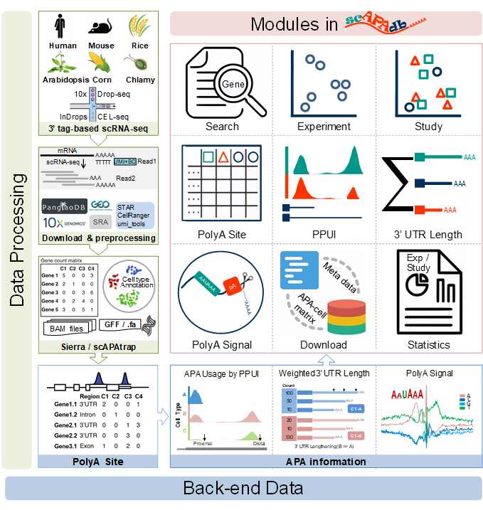
Schematic diagram of scAPAdb. (A) Data preprocessing and poly(A) site identification. (B) Back-end data of APA information stored in scAPAdb. (C) Functional modules in scAPAdb.
Gao, Y., et al. (2021) Analysis of alternative
polyadenylation from single-cell RNA-seq using scDaPars reveals
cell subpopulations invisible to gene expression, Genome Res.
Gruber, A.J. and Zavolan, M. (2019) Alternative cleavage and
polyadenylation in health and disease, Nature Reviews Genetics,
20, 1.
Hashimshony, T., et al. (2012) CEL-Seq: Single-Cell RNA-Seq
by Multiplexed Linear Amplification, Cell reports, 2, 666-673.
Levin, M., et al. (2020) Gene expression dynamics are a
proxy for selective pressures on alternatively polyadenylated
isoforms, Nucleic Acids Res, 48, 5926-5938.
Macosko, E.Z., et al. (2015) Highly Parallel Genome-wide
Expression Profiling of Individual Cells Using Nanoliter
Droplets, Cell, 161, 1202-1214.
Patrick, R., et al. (2020) Sierra: discovery of differential
transcript usage from polyA-captured single-cell RNA-seq data,
Genome Biol, 21, 167.
Shulman, E.D. and Elkon, R. (2019) Cell-type-specific
analysis of alternative polyadenylation using single-cell
transcriptomics data, Nucleic Acids Res, 47, 10027-10039.
Tian, B. and Manley, J.L. (2017) Alternative polyadenylation
of mRNA precursors, Nature reviews. Molecular cell biology, 18,
18-30.
Wu, X., et al. (2020) scAPAtrap: identification and
quantification of alternative polyadenylation sites from
single-cell RNA-seq data, Briefings in Bioinformatics.
Zheng, G.X., et al. (2017) Massively parallel digital
transcriptional profiling of single cells, Nature
communications, 8, 14049.
Ziegenhain, C., et al. (2017) Comparative Analysis of
Single-Cell RNA Sequencing Methods, Molecular cell, 65,
631-643.e634.
Cell Ranger : 3.1.0
STAR : 2.7.8a
samtools : 1.12
fastq-dump : 2.8.0
regtools : 0.5.2
umi¬_tools : 1.1.1
featureCounts : 2.0.1
DREME : 5.3.3
Install the following tools:
#Get STAR source using bioconda
conda install star -c bioconda

# Get Cell Ranger source from releases
wget -O cellranger-3.1.0.tar.gz "https://cf.10xgenomics.com/releases/cell-exp/cellranger-3.1.0.tar.gz?Expires=1627058816&Policy=eyJTdGF0ZW1lbnQiOlt7IlJlc291cmNlIjoiaHR0cHM6Ly9jZi4xMHhnZW5vbWljcy5jb20vcmVsZWFzZXMvY2VsbC1leHAvY2VsbHJhbmdlci0zLjEuMC50YXIuZ3oiLCJDb25kaXRpb24iOnsiRGF0ZUxlc3NUaGFuIjp7IkFXUzpFcG9jaFRpbWUiOjE2MjcwNTg4MTZ9fX1dfQ__&Signature=kW1lpq7UEJEcXttYKMcp9nvgQ6UsaVnNBQZ2eYjm29XCpMQMid-VAuk3PnbP97d54FinqT-8lsGnIr1ZKbBOu7WCJRsgc5GmbLI6jWg4EzsQje937iiL76v~Sp6LuVbfyLk~gzMyFPVipWYMcu3lXqWhkDHEFSZXYswF65ibAoaATakOJGNZvK2xD9Kb0JGpJRftkJppTVxBqtnQYpICVzlwFnVn8NJrrU8tjzcOwdFUPYMkWQhcvET1~aisJpHA8KeLU3Jg6XgbCDJ4m1ciy7koeoyuDR-hWNPGPiKWFyzFmp-5NiKGQ~10xBw3tM6oJSjlu~QEkMhTWKQpblgdJw__&Key-Pair-Id=APKAI7S6A5RYOXBWRPDA"

tar -xzvf cellranger-3.1.0.tar.gz
Motif analysis tool, DREME, is available as part of the MEME Suite of motif-based sequence analysis tools
# Get meme-5.3.3 source from releases
wget -c https://meme-suite.org/meme/meme-software/5.3.3/meme-5.3.3.tar.gz

#install meme-5.3.3
tar zxf meme-5.3.3.tar.gz
cd meme-5.3.3
./configure --prefix=$HOME/meme --enable-build-libxml2 --enable-build-libxslt
make
make test
make install
Make sure all tools are installed on your computer
#Get softwares source using bioconda
conda install samtools -c bioconda
conda install umi¬_tools -c bioconda
conda install regtools -c bioconda
conda install subread -c bioconda
You can install SRA Toolkit to download raw sequence data, and then use fastq-dump to turn convert sra format into fastq format. (SRA Toolkit includes prefetch and fastq-dump.)
#Get sra-tools source using bioconda
conda install sra-tools -c bioconda
#download reference genome
wget  –c ftp://ftp.ensemblgenomes.org/pub/plants/release-49/fasta/arabidopsis_thaliana/dna/Arabidopsis_thaliana.TAIR10.dna.toplevel.fa.gz
#download annotation gff3 file in gff3 format
wget –c ftp://ftp.ensemblgenomes.org/pub/plants/release-49/gtf/arabidopsis_thaliana/Arabidopsis_thaliana.TAIR10.49.gtf.gz
scRNA-seq data. We can download scRNA -seq data (fastq format) from public sequence repositories. For example, the data (SRR8257102) of Arabidopsis thaliana is downloaded from the Sequence Read Archive by SRA Toolkit.
#download sra
prefetch SRR8257102
#turn convert into fastq format
fastq-dump –O  /output-path/  SRR8257102.sra
Process fastq files
mv ./ SRR8257102_1.fastq ./ SRR8257102_S1_L001_R1_001.fastq
mv ./ SRR8257102_2.fastq ./ SRR8257102_S1_L001_R2_001.fastq
mv ./ SRR8257102_3.fastq ./ SRR8257102_S1_L001_I1_001.fastq
For Drop-seq or CEL-seq2 data, we need to use umi_tools to extract barcodes and umis to read_id. (using --bc-pattern=CCCCCCCCNNNN for Cel-seq2 data).
umi_tools extract --bc-pattern=CCCCCCCCCCCCNNNNNNNN --stdin ./ SRR8206654_1.fastq \
--stdout ./ SRR8206654_1_extracted.fastq --read2-in ./ SRR8206654_2.fastq \
--read2-out=./ SRR8206654_2_extracted.fastq --filter-cell-barcode --whitelist ./barcodes.tsv
The output file "SRR82066544_2_extracted.fastq" will be used for sequence alignment with STAR.
STAR --runMode genomeGenerate \
   --runThreadN 16  \
   --genomeFastaFiles ./Arabidopsis_thaliana.TAIR10.dna.toplevel.fa \
   --genomeDir ./TAIR10
Then we can align the data to the reference genome. Here SRR8206654 is a drop-seq dataset.
STAR --runThreadN 18
   --genomeDir ./TAIR10/ \
   --readFilesIn ./ SRR8206654_2_extracted.fastq \
   --outFilterMultimapNmax 1 \
   --outSAMtype BAM SortedByCoordinate \
   --outFileNamePrefix SRR8206654
The output file "SRR8206654Aligned.sortedByCoord.out.bam" is the alignment result (in bam format).
cellranger mkref
   --genome=./cellranger_TAIR10 \
   --fasta=./Arabidopsis_thaliana.TAIR10.dna.toplevel.fa \
   --genes=./Arabidopsis_thaliana.TAIR10.49.gtf \
   --nthreads=30
Then we can align the data to the reference genome.
cellranger count --id=run_tair_SRR8257102 \
   --fastqs=./fastqs/ \
   --transcriptome=./ cellranger_TAIR10 \
   --nosecondary
The output file "run_tair_SRR8257102/outs/possorted_genome_bam.bam" is the alignment result (in bam format).
Rscript ./scAPAtrap.R TENX sample-name bam-file barcodes-file read-lengthFor example:
Rscript ./scAPAtrap.R TENX SRR8257102 ./run_tair_SRR8257102/outs/possorted_genome_bam.bam ./barcodes.tsv 115
bash ./Sierra.sh ./Sierra.R bam-file barcodes-file GTF-file sample-name threadsFor example:
bash ./Sierra.sh ./Sierra.R ./ possorted_genome_bam.bam ./barcodes.tsv ../cellranger_TAIR10/gene/genes.gtf SRR8257102 24The output file “SRR8257102_peaks_annotation.txt” is the result and we use this file for further process.
  ## path is the address path of sierra's output file
  ## gtf is the corresponding annotation gtf file path
  library(movAPA)
  dirlist <- dir(path)
  peakdir <- dirlist[grep("_peak_annotations.txt",dirlist)]
  countdir <- dirlist[grep("_count$",dirlist)]

  peak_annotations <- read.delim(paste0(path,"/",peakdir))
  peak_annotations$coord <- 0
  peak_annotations[peak_annotations$strand == "+",]$coord <- peak_annotations[peak_annotations$strand == "+",]$end
  peak_annotations[peak_annotations$strand == "-",]$coord <- peak_annotations[peak_annotations$strand == "-",]$start

  peak_annotations$seqnames

  PACds <- peak_annotations[,c("seqnames","start","end","strand","coord","gene_id")]
  colnames(PACds) <- c("chr","start","end","strand","coord","gene_id")
  PACds <- unique(PACds)
  anno <- annotatePAC(PACds, aGFF = gtf)
  anno <- arrange(anno, chr,ftr_start)

  count <- ReadPeakCounts(paste0(path,countdir,"/"))
  count <- as.data.frame(count)
  intpas <- rownames(anno)[rownames(anno) %in% rownames(count)]

  count <- count[intpas,]
  anno <- anno[intpas,]
  anno$gene_range <- rownames(anno)
  anno$gene <- gsub("[.].*","",anno$gene)
  anno <- anno[!is.na(anno$gene),]
  p <- readPACds(anno, colDataFile=NULL,noIntergenic=FALSE)
  p@anno$ftr_raw <- p@anno$ftr
  p <- ext3UTRPACds(p, 1000)

  panno <- arrange(p@anno, chr,ftr_start)

  count <- count[panno$gene_range,]
  rownames(count) <- rownames(panno)
  puni <- unique(panno[,c("chr","coord","strand","ftr","gene")])

  colnames(count) <- gsub("-.*","",colnames(count))
  p@counts <- count[rownames(puni),]
  p@anno <- panno[rownames(puni),]
We use the movAPA R package to annotate poly(A) sites.
The GTF file we use is the latest minor version of the
GTF file for sequence alignment.library(movAPA)
gff<-parseGenomeAnnotation(“./Arabidopsis_thaliana.TAIR10.49.gtf”)
##Make sure chromosomes in scPACds are consistent with that in gff.
gff$anno.need$seqnames<-paste0("chr",gff$anno.need$seqnames)
gff$anno.rna$seqnames<-paste0("chr",gff$anno.rna$seqnames)
gff$anno.frame$seqnames<-paste0("chr",gff$anno.frame$seqnames)
load(“SRR8257102_APA.Rda”)
scPACds <- annotatePAC(scPACds,gff)
scPACds <- ext3UTRPACds(scPACds,ext3UTRlen = 1000)
new_annos <- annoMergePA(pa_anno,refPAS,"GSM2803334")
pa_annoNew <- new_annos[[1]]
new_refPAS <- new_annos[[2]]

## input
# pa_anno: the pa meta of an experiment
# annoDB: the reference PAS dataset
# source_name: the name of this polyA sites source
# obs: The deviation value of the intersection of the comparison ranges
## output
# pa_anno: The updated pa meta
# annoDB: The updated reference PAS dataset, and subsequent experiments can be matched based on this updated reference PAS dataset.

annoMergePA <- function(pa_anno,annoDB,source_name,obs=10){

  pb <- txtProgressBar(style=3)
  star_time <- Sys.time()

  pa_anno$PA_id <- paste0("PA:",pa_anno$gene,":",pa_anno$coord)
  pa_anno$PA_id2 <- pa_anno$PA_id
  pa_anno$gene <- toupper(pa_anno$gene)
  annoDB$gene_id <-  toupper(annoDB$gene_id)
  sub_anno <- pa_anno[(pa_anno$gene %in% annoDB$gene_id),]

  #Judging whether there is an intersection by interval
  for(i in 1:nrow(sub_anno)){
    setTxtProgressBar(pb, i/nrow(sub_anno))

    gene_id <- sub_anno[i,]$gene
    coord <- sub_anno[i,]$coord
    start <- sub_anno[i,]$start
    end <- sub_anno[i,]$end
    ftr <- sub_anno[i,]$ftr
    PA_id <- sub_anno[i,]$PA_id
    ftr_start <- sub_anno[i,]$ftr_start
    ftr_end <- sub_anno[i,]$ftr_end
    sub_db <- annoDB[annoDB$gene_id == gene_id,]
    ref_start <- sub_db$start
    ref_end <- sub_db$end
    ranks <- rank(ref_start)
    ref_start <- ref_start[ranks] -obs
    ref_end <- ref_end[ranks] +obs
    loc <- ref_start < end & ref_end > start
    if(sum(loc) == 1){

      sub_anno[i,]$PA_id2 <- sub_db[ranks,]$PA_id[loc]
    }else if(sum(loc) > 1){

      ref_coord <- as.numeric(sub_db[ranks,]$coord[loc])
      loc2 <- which.min(abs(ref_coord-coord))
      sub_anno[i,]$PA_id2 <- sub_db[ranks,]$PA_id[loc][loc2]
    }else{
      dt <- sub_db[1,]
      dt$PA_id <- PA_id
      dt$start <- start
      dt$end <- end
      dt$coord <- coord
      dt$ftr_start <- ftr_start
      dt$ftr_end <- ftr_end
      dt$source <- source_name
      annoDB <- rbind(annoDB,dt)
    }
  }

  locs <- match(rownames(sub_anno),rownames(pa_anno))
  pa_anno$PA_id2[locs] <- sub_anno$PA_id2

  No_anno <- pa_anno[!(pa_anno$gene %in% annoDB$gene_id),]
  new_anno <- No_anno[,c("PA_id","chr","start","end","strand","coord","ftr","gene","ftr_start","ftr_end")]

  if(nrow(new_anno) >1){
    new_anno$source <- source_name
    colnames(new_anno)<- colnames(annoDB)
    annoDB <- rbind(annoDB,new_anno)
  }

  end_time <- Sys.time()
  close(pb)
  run_time <- end_time - star_time
  return(list(pa_anno,annoDB))
}
~/meme/bin/dreme -oc ./motif/up50nt -p ./fasta/ SRR8257102.up50nt.fa -k 6
~/meme/bin/dreme -oc ./motif/dn50nt -p ./fasta/ SRR8257102.dn50nt.fa -k 6
~/meme/bin/dreme -oc ./motif/upFar50nt -p ./fasta/ SRR8257102.upFar50nt.fa -k 6
In scAPAdb, we catalog APA datasets by experiments and
studies,
respectively. An experiment is a dataset from cells originating
from
the same common biological source or sequencing experiment,
which is
normally a GEO sample (accession in the form of GSM#) or an SRA
experiment (accession in the form of SRX#). A study is a dataset
containing multiple experiments, which is normally represented
as a
GEO data series (accession in the form of GSE#) or an SRA study
(accession in the form of SRA#).
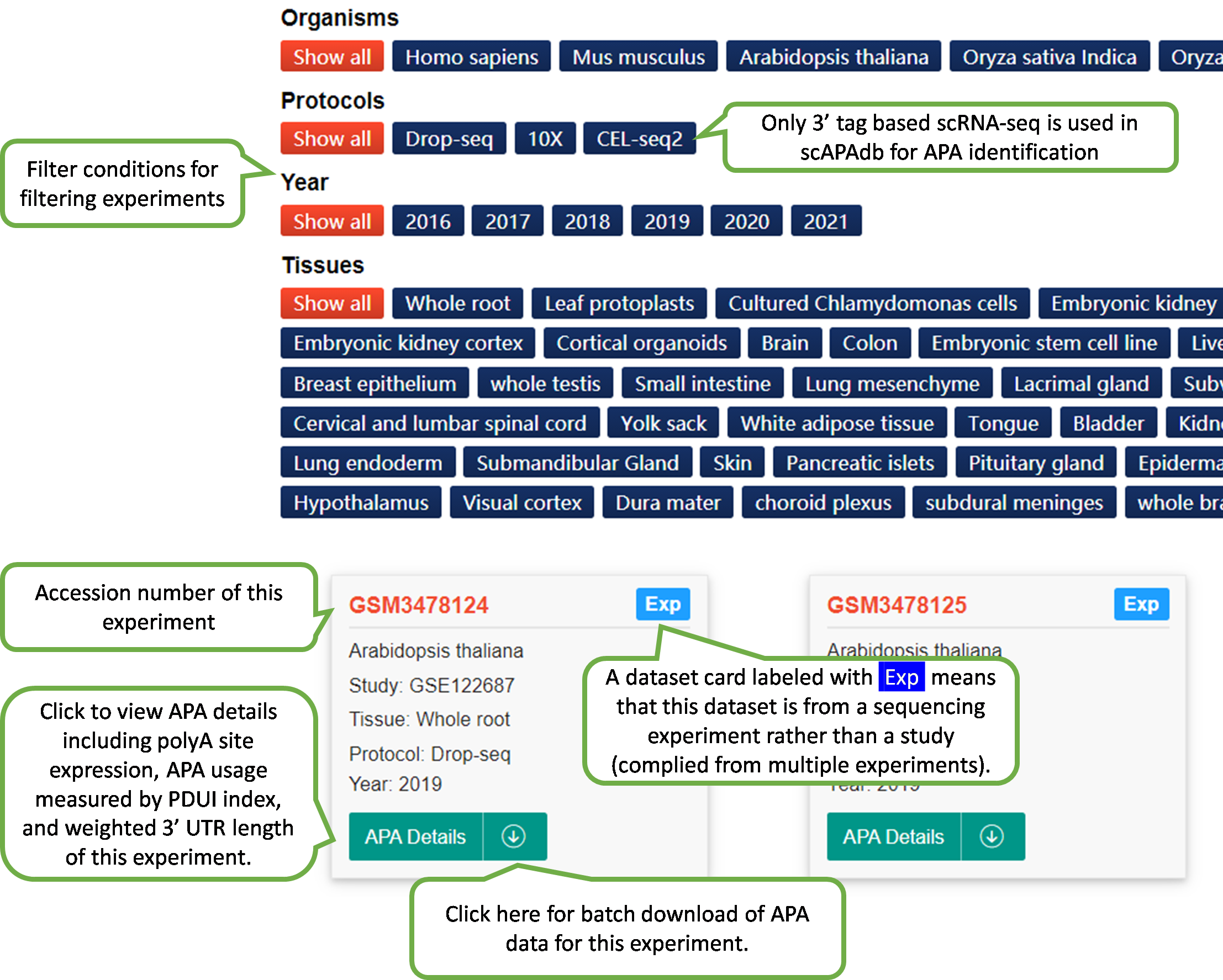
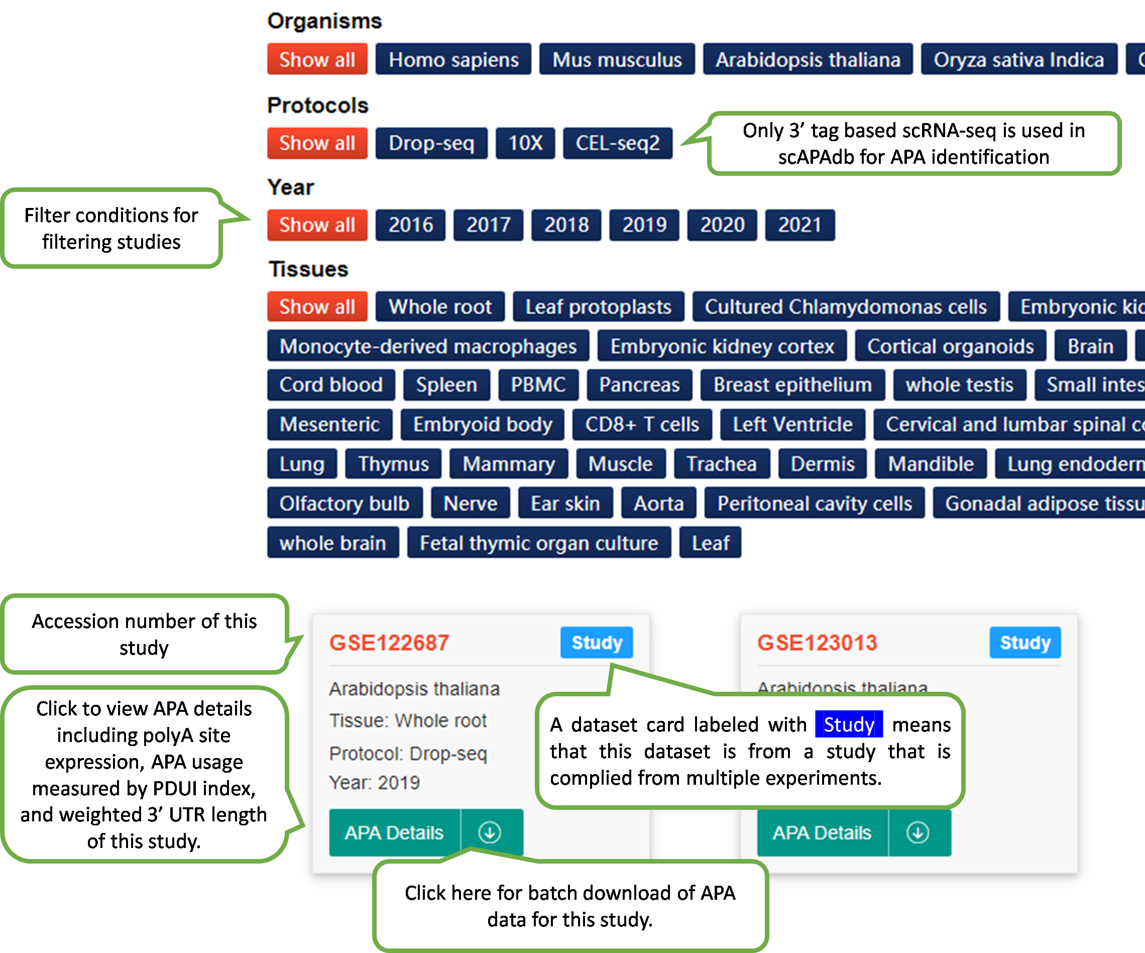
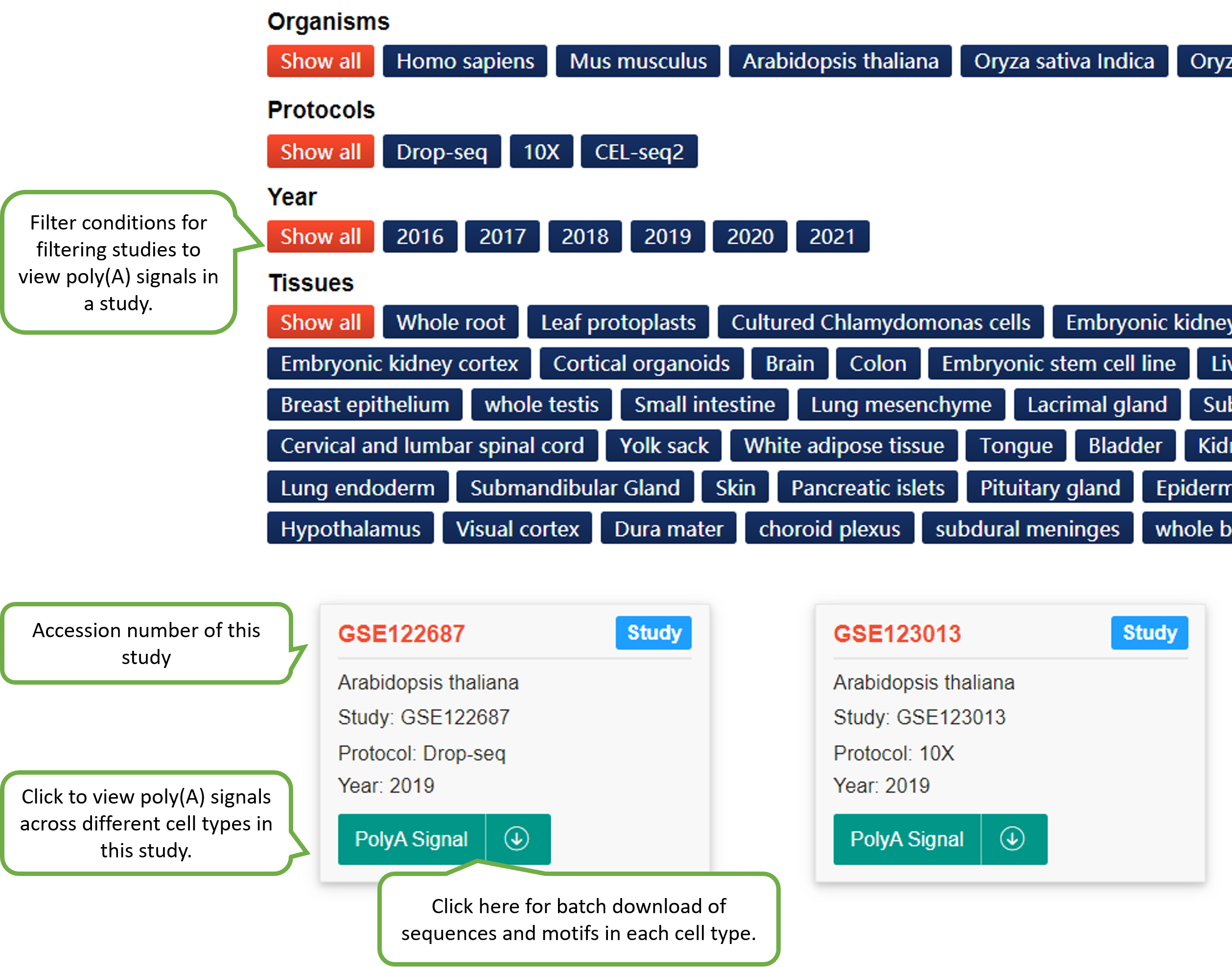
In scAPAdb, the Experiment page catalogs
APA
datasets by
experiments, which can be filtered by different categories such
as
species, date of publish, sequencing protocol and tissue.
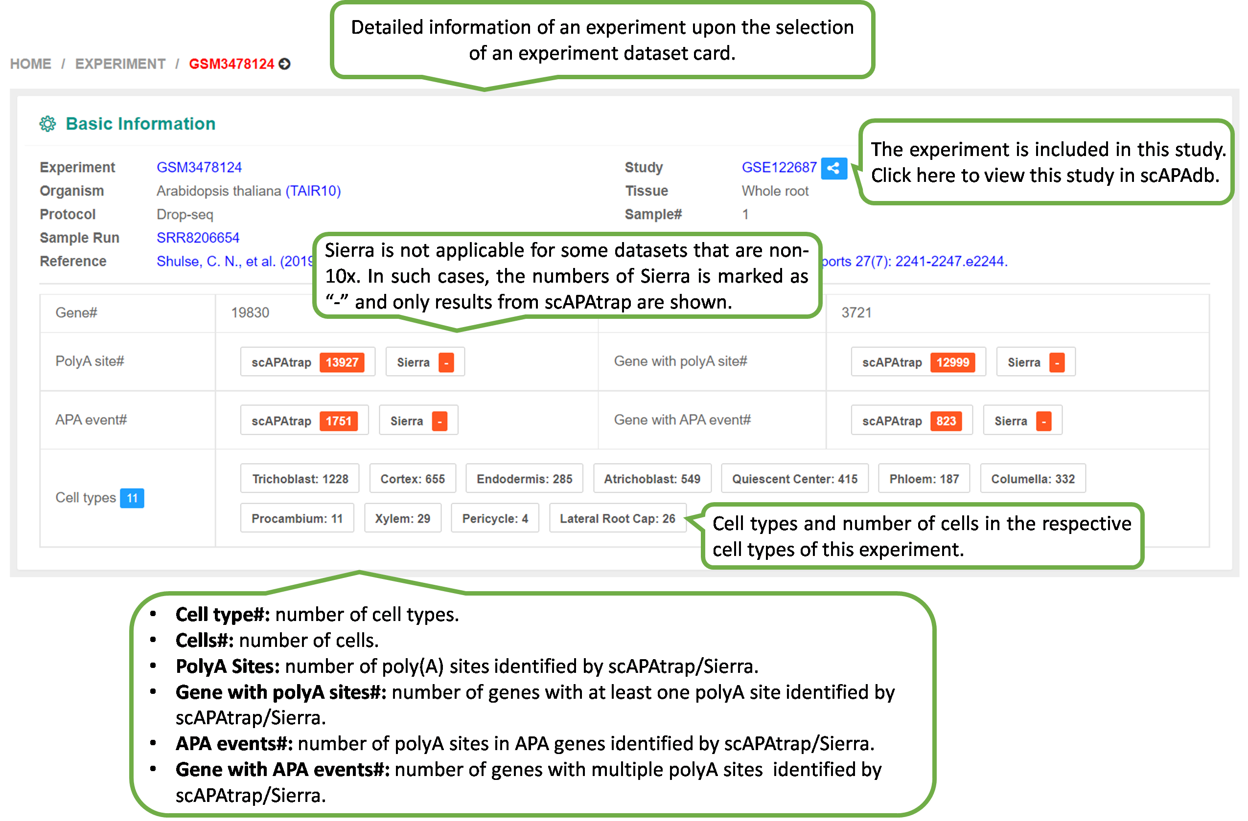
The webpage of detailed information of an experiment will be
shown upon the selection of an experiment dataset card.
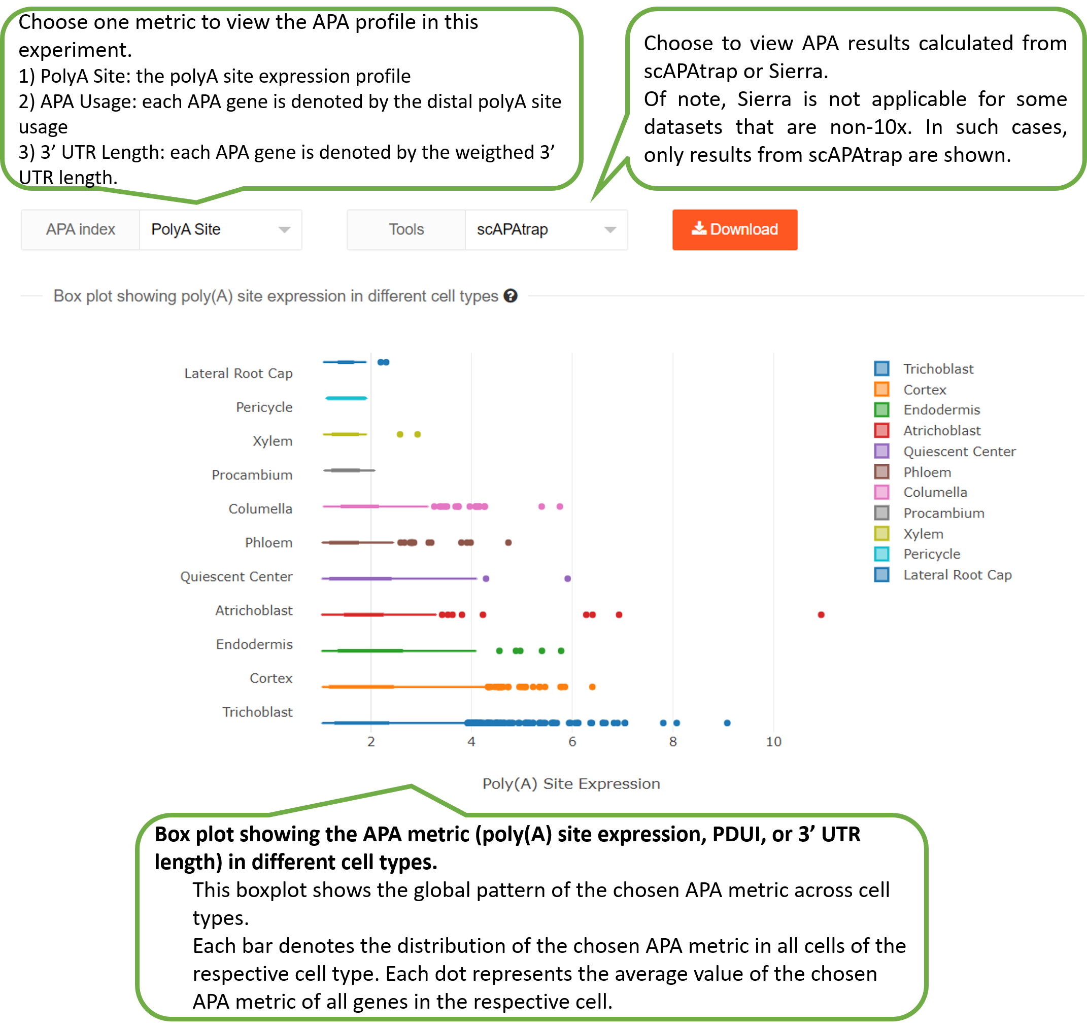
The "Experiment" page provides three metrics computed by
scAPAtrap and/or Sierra to characterize the APA profile in
this
experiment:
1) PolyA Site: the polyA site expression profile.
2) APA Usage: each APA gene is denoted by the distal polyA
site
usage.
3) 3' UTR Length: each APA gene is denoted by the weigthed
3'
UTR length.
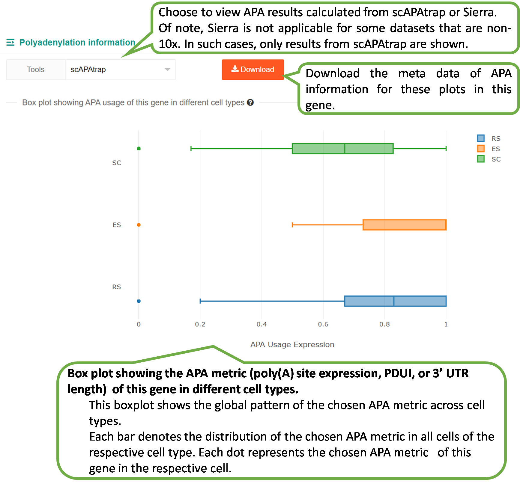
Of note, Sierra is not applicable for some datasets that are
non-10x, therefore, only results from scAPAtrap are
shown.
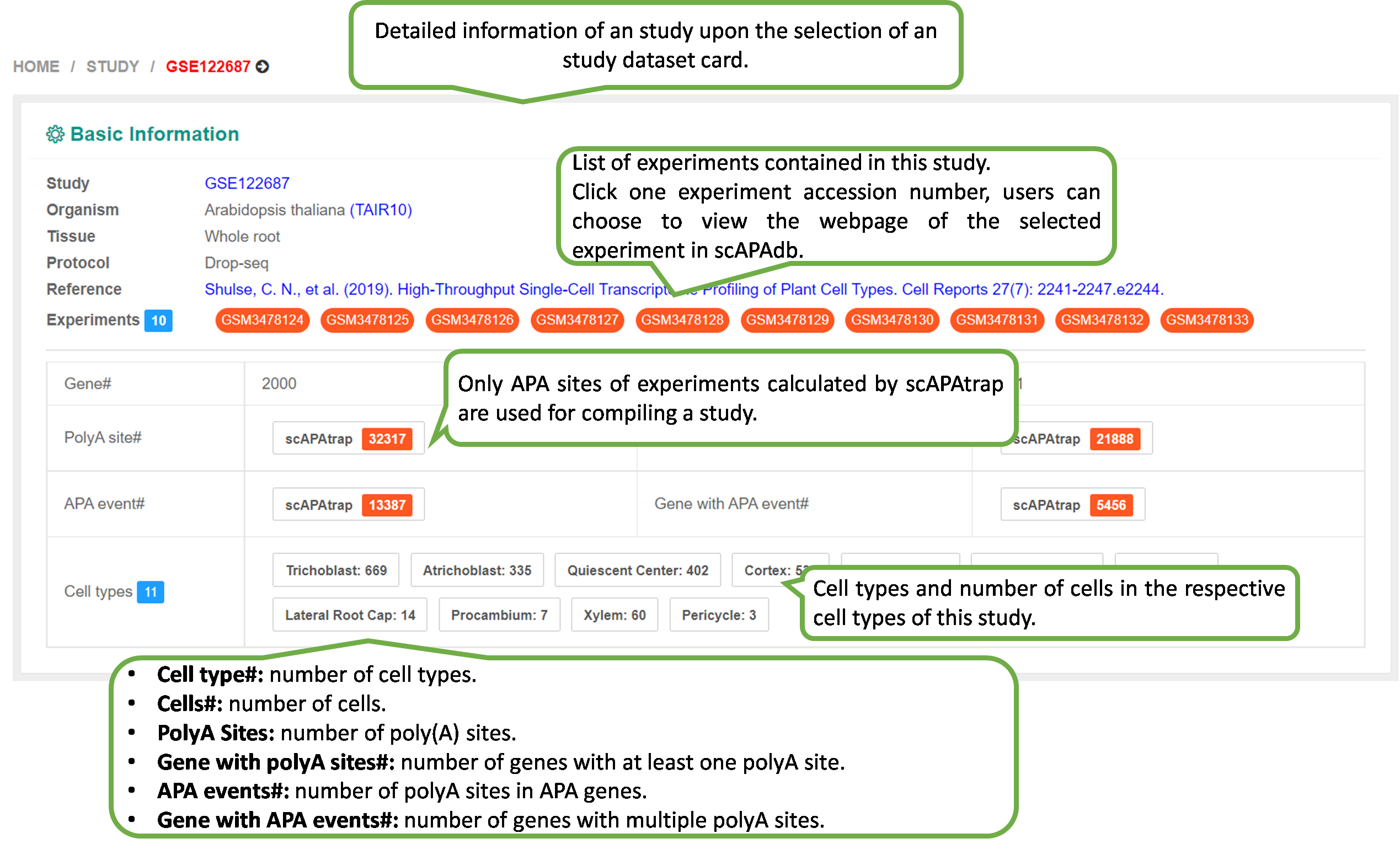
In scAPAdb, we catalog APA datasets by experiments and studies, respectively. An experiment is a dataset from cells originating from the same common biological source or sequencing experiment, which is normally a GEO sample (accession in the form of GSM#) or an SRA experiment (accession in the form of SRX#). A study is a dataset containing multiple experiments, which is normally represented as a GEO data series (accession in the form of GSE#) or an SRA study (accession in the form of SRA#). To compile an APA atlas for a study, poly(A) sites from individual experiments of scAPAtrap were annotated with the reference poly(A) sites and then merged into a consensus list.
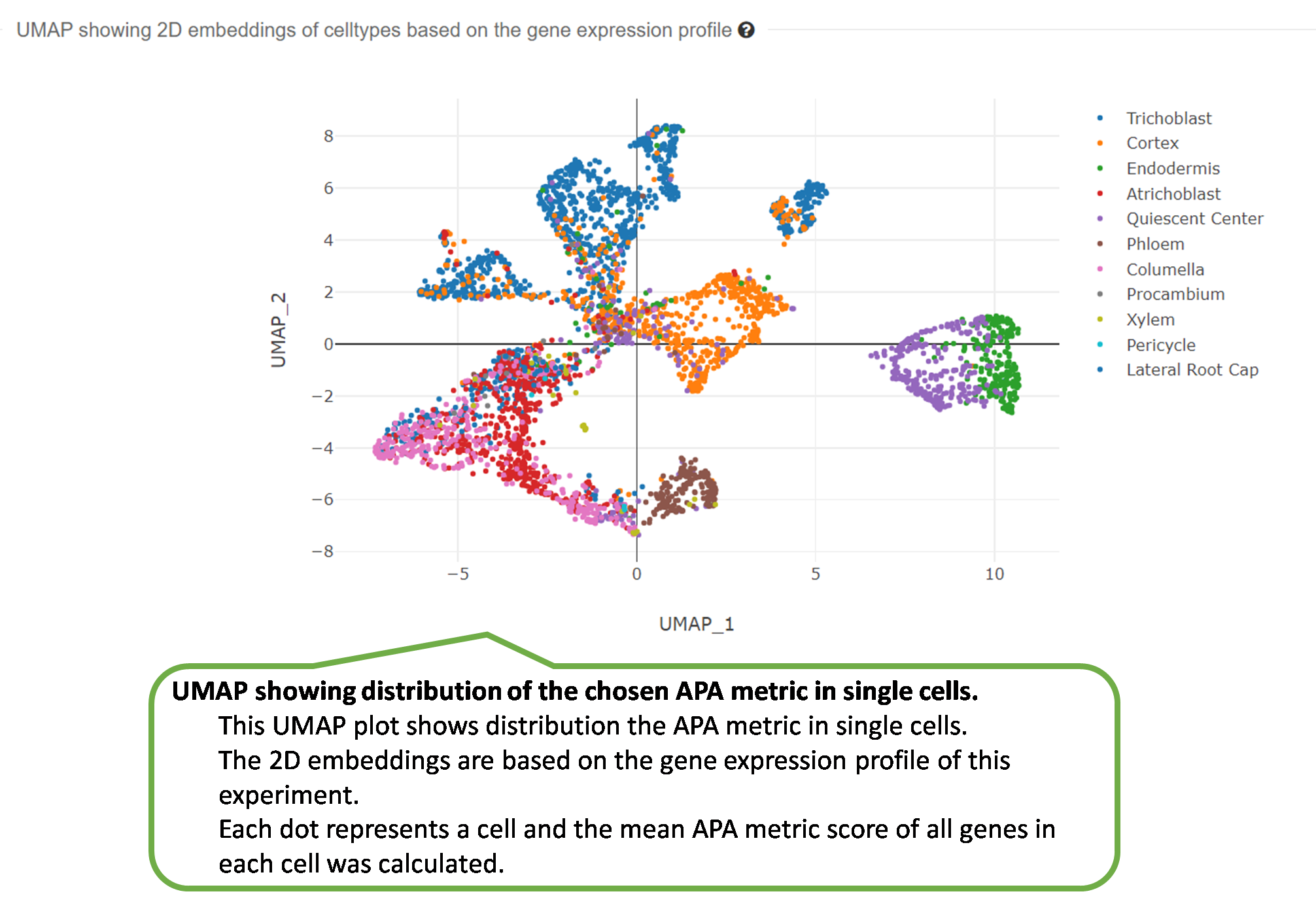
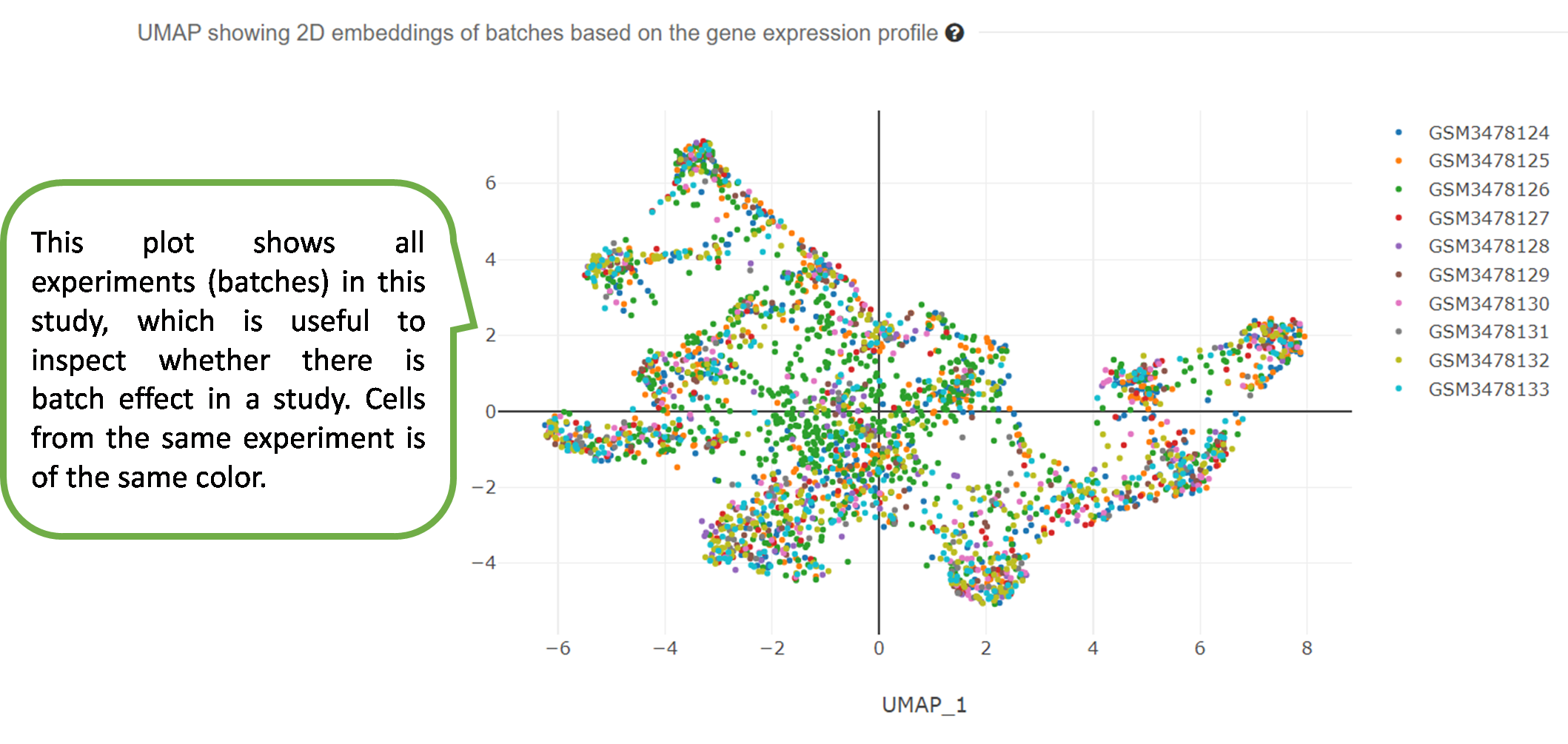
Similar to the Experiment results, the following four plots
are
shown for each study. Please see the
for detailed explanation.
1) Box plot showing one APA metric (poly(A) site expression,
PPUI, or 3' UTR length) in different cell types.
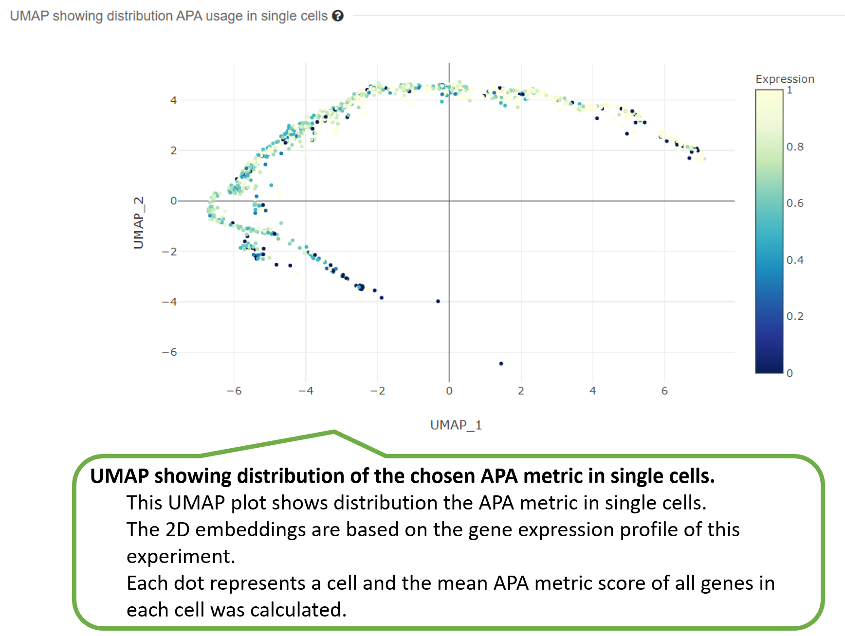
2) UMAP showing distribution of one APA metric in single
cells.
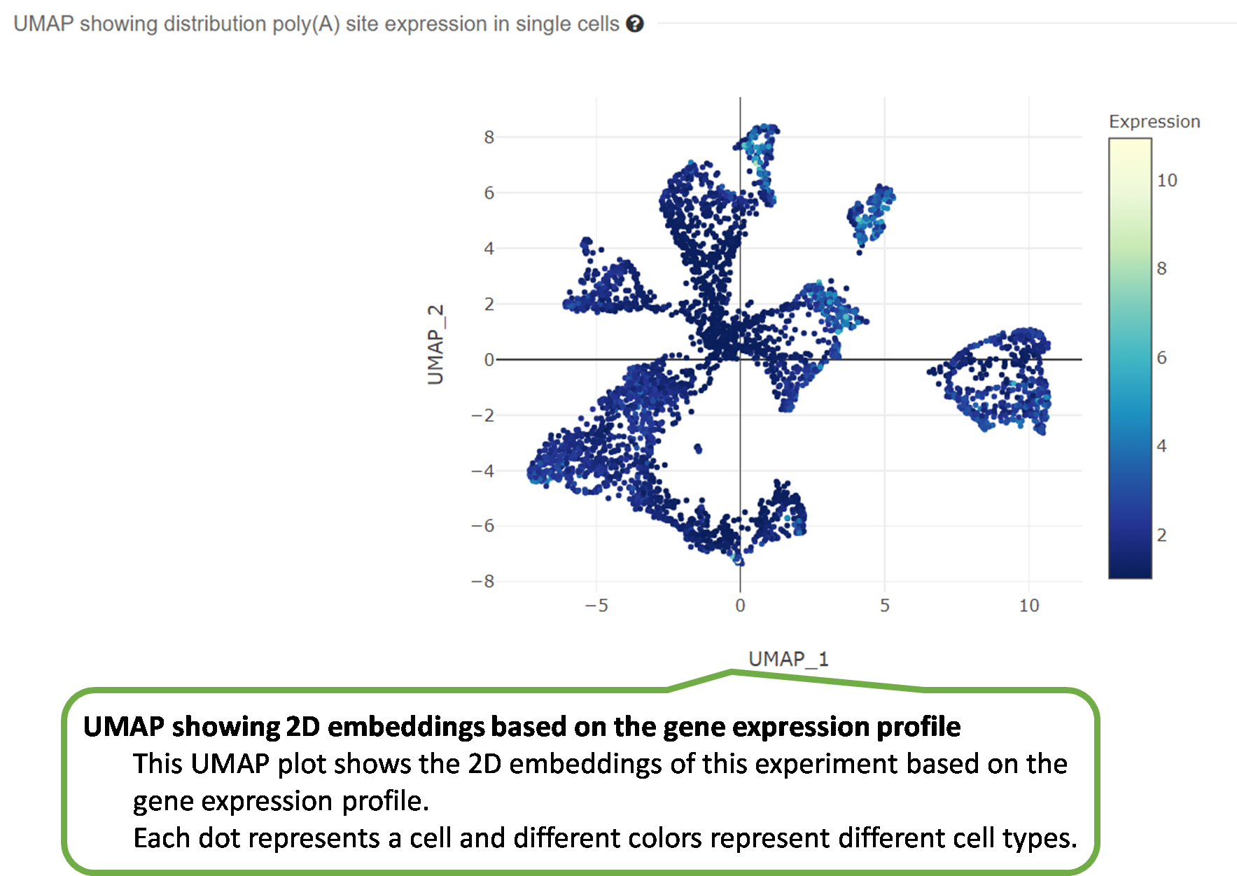
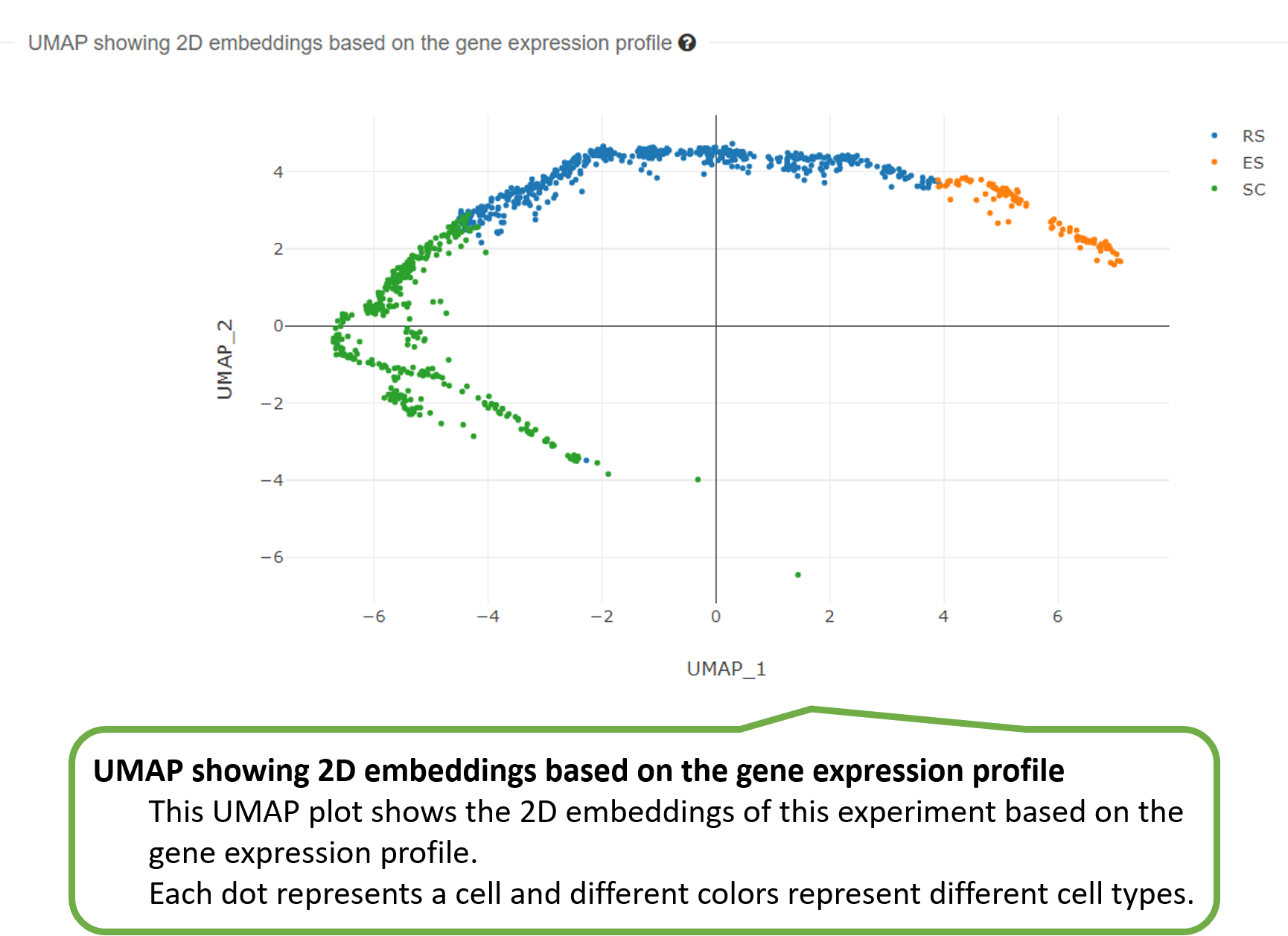
3) UMAP showing 2D embeddings based on the gene expression
profile.
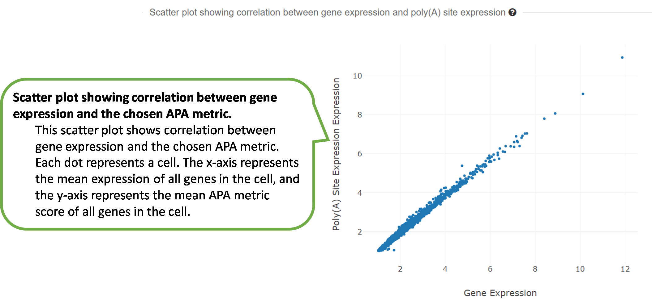
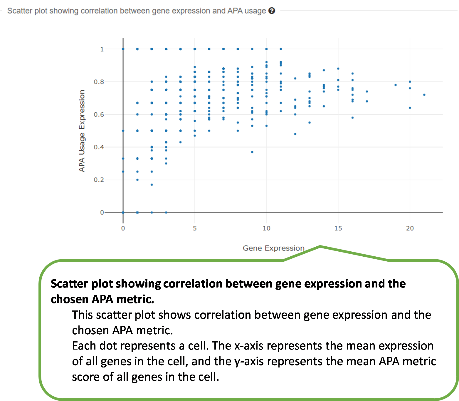
4) Scatter plot showing correlation between gene expression
and
the selected APA metric.
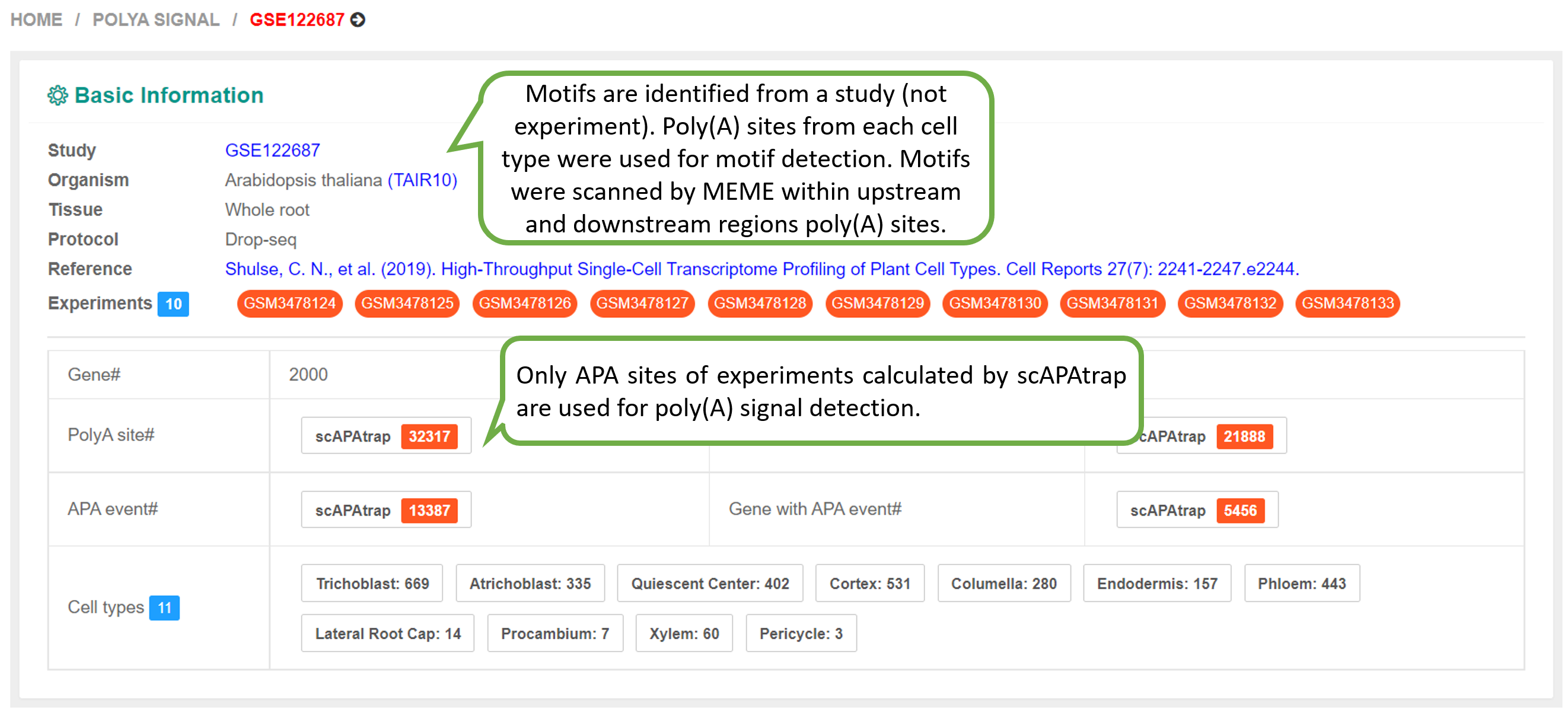
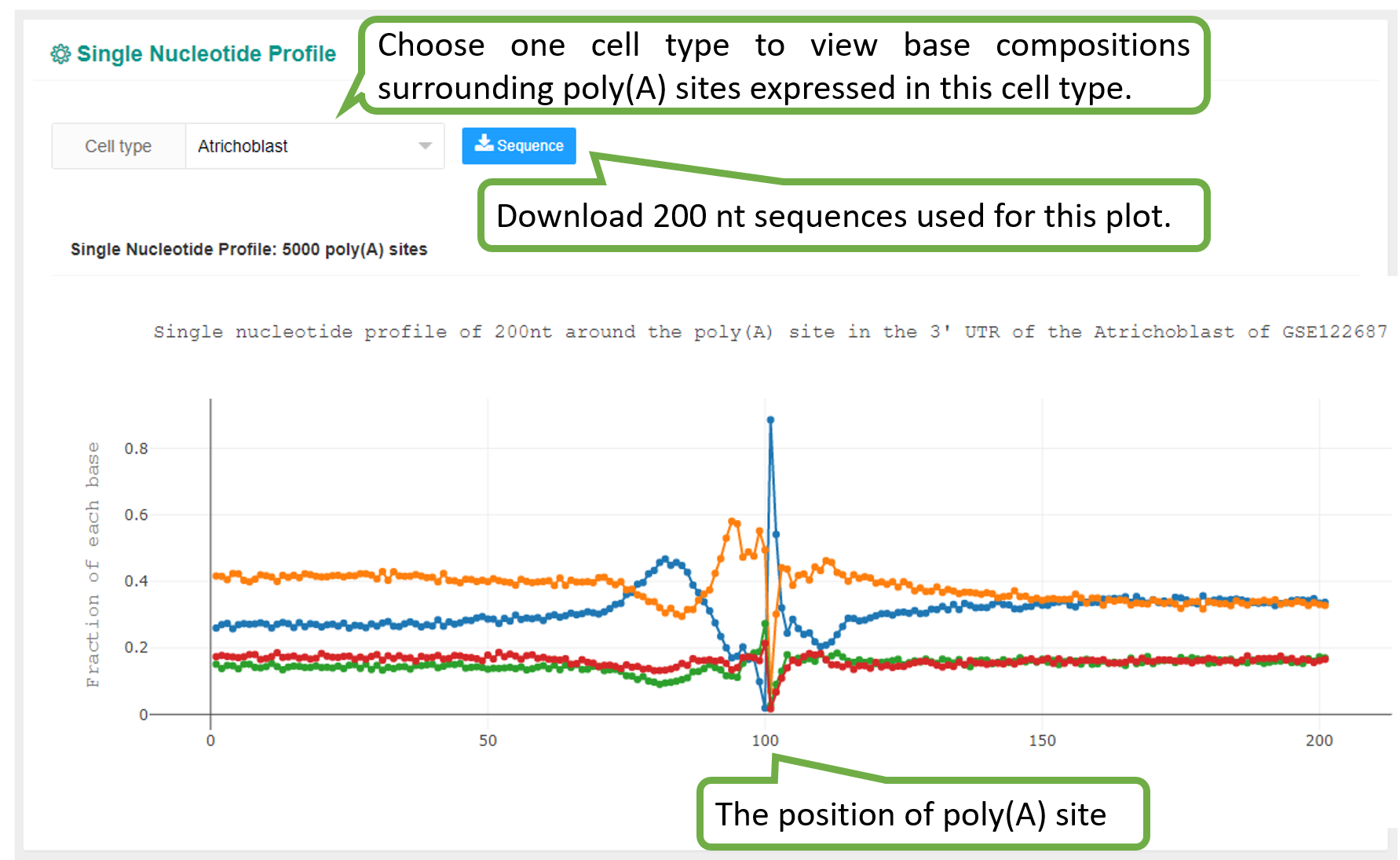
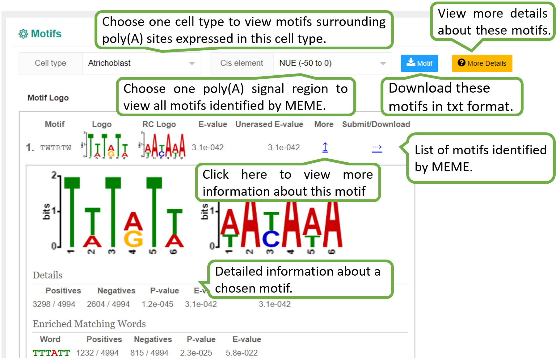
We identified poly(A) signals for each cell type in each study of each species. Given the PA-matrix of each study, poly(A) sites expressed in each cell type were filtered and ordered by the expression level. To speed up calculation, if the number of poly(A) sites expressed in a cell type is higher than 5000, then only the top 5000 sites were retained for motif analysis. Sequences surrounding poly(A) sites (-200 to 200 nt) were extracted and single nucleotide compositions around poly(A) sites were calculated. The DREME function of MEME with default options (E-value threshold=0.05) was adopted to search motifs significantly enriched within the near upstream (-50 to 0 nt), far upstream (-50 to -100 nt) and downstream (0 to 50 nt) of poly(A) sites. According to previous studies on poly(A) signals, pentamers were searched for Chlamy and hexamers were searched for other species. Since scAPAtrap can determine the exact location of poly(A) sites by using the strategy of poly(A) read anchoring, we only used poly(A) sites identified by scAPAtrap for poly(A) signal identification.
The PolyA Site, APA Usage and 3' UTR Length pages
under the
APA index menu provide APA information in individual cells of
each experiment, including poly(A) sites identified by scAPAtrap
and Sierra, PPUI scores of APA genes and the weighted 3' UTR
length (WUL) of APA genes.
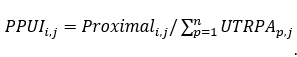
The PPUI of poly(A) site i in cell j is calculated as the ratio of expression level of the proximal site to the sum of expression levels of all 3' UTR sites in the respective gene in sample j:
Given a gene with at least two polyA sites in 3' UTR, then WUL score can be calculated. For example, geneX has three polyA sites in 3' UTR. First we calculated the distance from each polyA site to the stop codon. Then
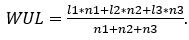
| geneX | Distance to stop codon | Number of supported reads |
|---|---|---|
| PA1 | l1 | n1 |
| PA2 | l2 | n2 |
| PA3 | l3 | n3 |
For a given experiment, PPUI or WUL scores of a given gene or
the
overall score of all genes in individual cells are present,
which
can reflect APA dynamics (3' UTR shortening/lengthening) across
cell
types. A smaller PPUI or higher WUL means 3' UTR lengthening,
i.e.,
higher usage of the distal poly(A) site. For instance, on the
"Experiment" page of GSM2803334
showing one sample of the mouse
sperm study, the overall distribution of mean PPUI scores of all
genes in individual cells was visualized by UMAP and bar plot,
which
reflects the gradual shortening of 3' UTR in the transition from
spermatocytes (SC) to elongating spermatids (ES).
Plots of "PolyA Site", "APA Usage" and "3' UTR length" in an
experiment are similar. Please refer to for details.
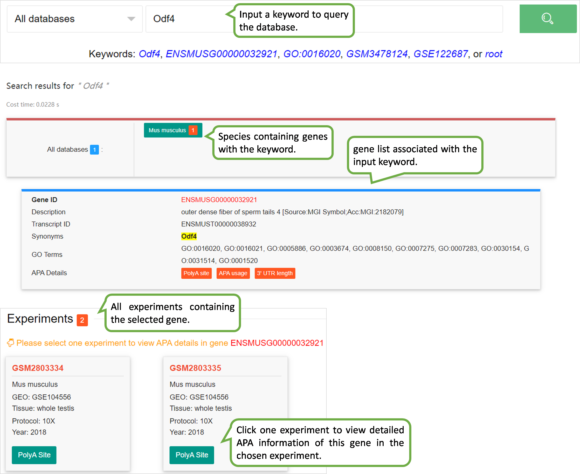
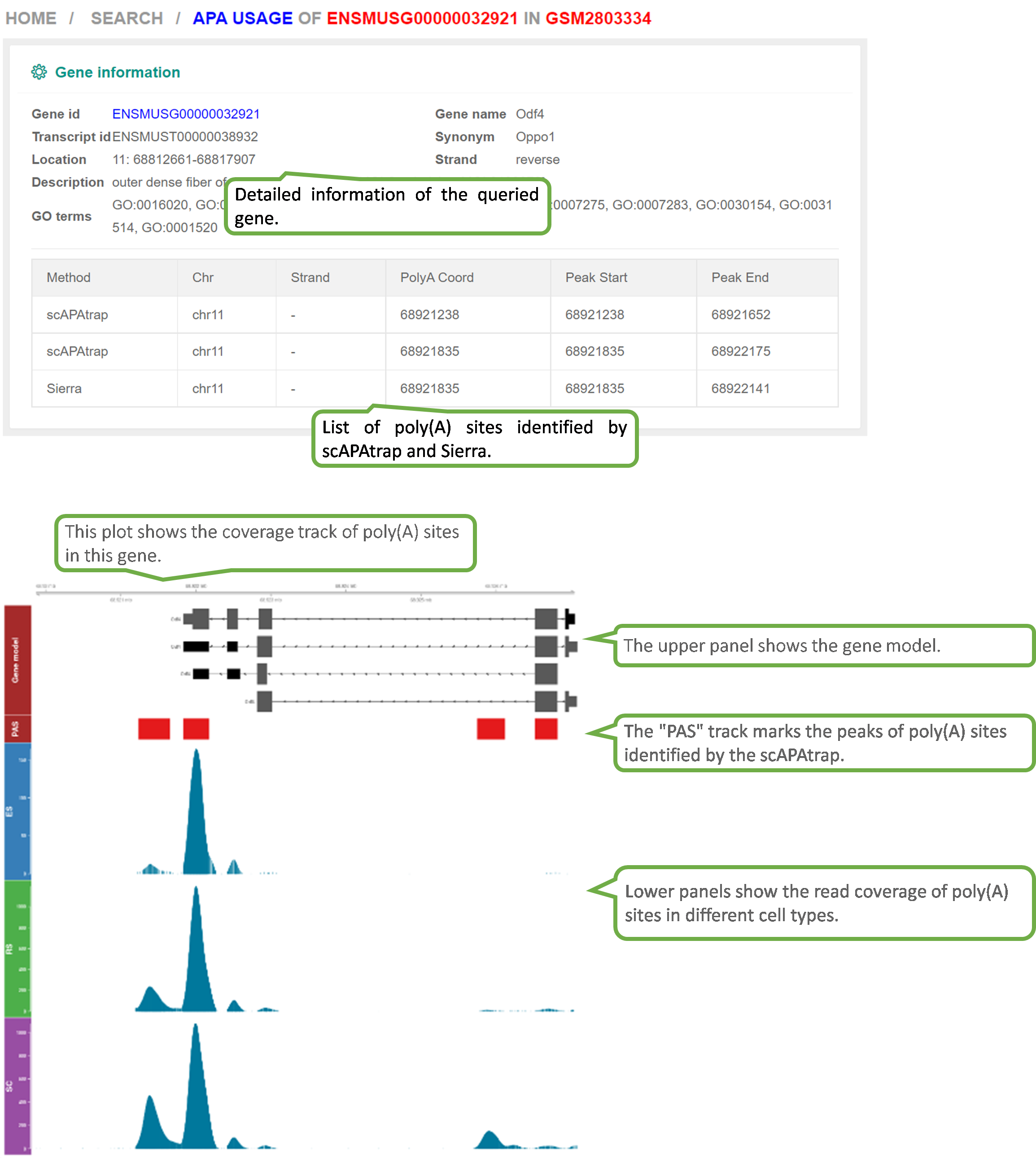
scAPAdb provides a very convenient search interface for querying gene(s) by commonly used keywords such as gene identifier, gene symbol/alias, gene description, gene function, and gene ontology (GO) ID. Users can also search an experiment or a study by an accession number. A query with gene relevant keywords will lead to an intermediate page showing the experiments with at least one poly(A) site identified in the queried gene(s). Then users can choose to view the full APA information of the queried gene in a selected experiment. A query with accession number will directly lead to the page of the quired experiment or study. Take the Odf4 gene for example, which has been reported to play an important role in sperm tails. After searching for this gene in the database, an intermediate page opens, which shows a detailed gene list associated with the input keyword. By clicking the gene of interest (here is ENSMUSG00000032921), a new page opens to show all experiments containing this gene. By clicking the dataset card of the experiment GSM2803334, detailed information of the gene and the usage of poly(A) sites across cell types. Two poly(A) sites were detected in the 3 UTR and extended 3 UTR of this gene by scAPAtrap, whereas only one poly(A) site was identified by Sierra. The read coverage of the distal poly(A) site in this gene is increased from SC to ES, suggesting the APA dynamics of 3 UTR shortening during mouse spermatogenesis. APA dynamics across cell types quantified by the PPUI or WUL score also reflect the gradual 3' UTR shortening in the transition from SC to ES. The scatter plot shows the correlation between the profile of the APA usage and gene expression.
The Download page provides
batch download of data in the database. For each experiment or
study, different files are available for download to meet the
users' needs.
An experiment is a dataset from cells originating from the same
common biological source or sequencing experiment, which is
normally a GEO sample (accession in the form of GSM#) or a SRA
experiment (accession in the form of SRX#).
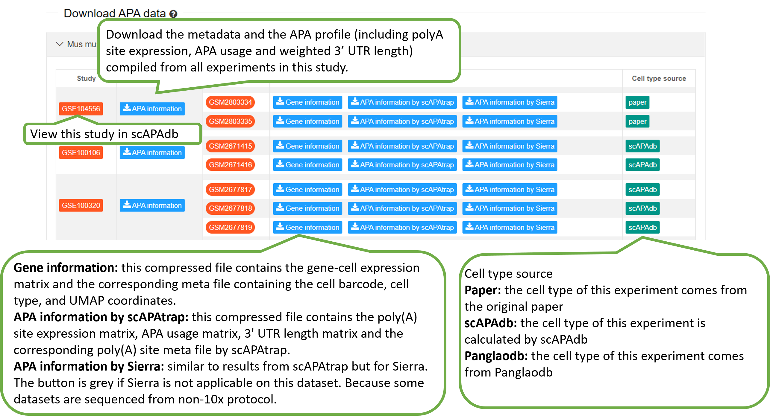
For each experiment, we provided the following files for download, including the gene-cell expression matrix, the metafile, the poly(A) site files generated by scAPAtrap and Sierra.
| gene.csv | The gene-cell expression matrix, with each row being a gene and each column being a cell. This file is normally obtained from public database like PanglaoDB, otherwise it is generated by tools like CellRanger. |
| meta.csv | The meta file containing the cell barcode, cell type, and UMAP coordinates. |
For either scAPAtrap or Sierra, we provided the following files for download.
| polyasite_counts.csv | The poly(A) site expression matrix, with each row being a poly(A) site and each column being a cell. The value is the poly(A) site expression denoted by the number of supported 3' reads. |
| usage_counts.csv | The PPUI matrix containing the relative usage of the proximal poly(A) site, with each row being a gene and each column being a cell. The value is the PPUI score. Only genes with at least two poly(A) sites in 3' UTR or extended 3' UTR were used. |
| length_counts.csv | The WUL matrix containing the weighted 3' UTR length, with each row being a gene and each column being a cell. The value is the weighted 3' UTR length. Only genes with at least two poly(A) sites in 3' UTR or extended 3' UTR were used. |
| pa_meta.csv | The meta file recording the annotation of poly(A)
sites,
with each row being a poly(A) site. This matrix
includes the
following columns:
|
A study is a dataset complied from multiple experiments, which is normally represented as a GEO data series (accession in the form of GSE#) or a SRA study (accession in the form of SRA#). The current version of scAPAdb provides the atlas of poly(A) sites compiled from results of scAPAtrap. For each study, we provided the following files for download, including the metafile, the poly(A) site files compiled from different experiments.
| barcodes.csv | The meta file containing the cell barcode, batch of an experiment, and cell type labels. |
| Integrate_counts.csv | The compiled gene-cell expression matrix, with each row being a gene and each column being a cell. |
| polyasite_counts.csv | The compiled poly(A) site expression matrix, with each row being a poly(A) site and each column being a cell. The value is the poly(A) site expression denoted by the number of supported 3' reads. |
| usage_counts.csv | The compiled PPUI matrix containing the relative usage of the proximal poly(A) site, with each row being a gene and each column being a cell. The value is the PPUI score. Only genes with at least two poly(A) sites in 3' UTR or extended 3' UTR were used. |
| length_counts.csv | The compiled WUL matrix containing the weighted 3' UTR length, with each row being a gene and each column being a cell. The value is the weighted 3' UTR length. Only genes with at least two poly(A) sites in 3' UTR or extended 3' UTR were used. |
| pa_meta.csv | pa_meta.csv is only the high variable polyA sites
obtained by applying Seurat's FindVariableFeatures
on the polysite_counts matrix (similar to HVGs of
the Seurat package). The names of these polyA sites
have been unified by matching to reference PAS
datasets. This matrix includes the following
columns:
|
In addition to the APA content, the full list of the reference genome assembly and genome annotation for each species, and relevant bioinformatics workflows used in scAPAdb are also described.
To compile an APA atlas for a study, we used known polyA sites
collected from bulk 3′-seq as the reference to annotate polyA
sites from scRNA-seq.
The Download page provides reference PAS datasets of different
species that we have prepared.
Each reference PAS dataset contains the following information.
| PA_id | The id of the polyA site after integration, which is composed of "PA", gene id, and coord |
| chr | The chromosome name |
| start | The start position of the poly(A) site cluster |
| end | The end position of the poly(A) site cluster |
| strand | The strand of "+" or "-" |
| coord | The coordinate of the polyA site |
| ftr | The gene region where polyA site is located. |
| gene_id | the gene id |
| source | The annotation source of this polyA site |
1. How the cell types are annotated in scAPAdb?
The R scripts and related resources for cell type annotation are provided here.
In scAPAdb, we tried to collect cell type labels from original papers or public resource platforms like PanglaoDB, however, there are still many papers that did not provide cell type annotation files. In such cases, we inferred cell types from the gene-cell expression matrix using computational pipelines. Generally, cell type information in scAPAdb is mainly obtained by the following three sources: i) cell type information provided in the original paper (if any); ii) cell type information provided in PanglaoDB (if any); iii) collecting as many marker genes as possible from CellMarker (Zhang, et al., 2018), PanglaoDB, the source of the data and related papers, and then inferring cell types by computation. Among these species, the data of Arabidopsis mainly comes from several newly published papers. We referred to the annotation methods of two studies (Shahan, et al., 2020; Shulse, et al., 2019) to annotate cell types for each single cell rather than cell clusters. For other species, we cluster cells first by Seurat (Stuart, et al., 2019) and then annotate cell types by AUcell (Aibar, et al., 2017). For the PBMC (Peripheral blood mononuclear cell) data, in addition to marker genes from CellMarker and PanglaoDB, we also collected marker genes from some PBMC-related papers (Oksvold, et al., 2014; Sinha, et al., 2018; Zheng, et al., 2017).
For Arabidopsis, we basically followed the way in Shulse, et al. (Shulse, et al., 2019) to infer cell types, but we referred to Shahan, et al. (Shahan, et al., 2020) to infer cell type for each single cell rather than for each cell cluster. This is because that majority of scRNA-seq data in Arabidopsis are from the same tissue (root) and there are rich resources on bulk gene expression data, which provides sufficient information for inferring cell types for individual cells. We compiled gene markers from all current scRNA-seq studies on Arabidopsis, and collected bulk gene expression profiles from published microarray and RNA-seq data as reference (Brady, et al., 2007; Li, et al., 2016). Then we inferred the cell type for each cell by three ways as in (Shulse, et al., 2019). i) We calculated the Pearson correlation coefficient between the expression profile of each cell and the reference gene expression profile. ii) We combined the cell-type specific gene expression profiles available in Arabidopsis Gene Expression Database (AREX: http://www.arexdb.org) (also provided in (Shahan, et al., 2020)) to compute the ICI (index of cell identity) score of each cell to quantify the relative weight of each cell type. iii) We used AUCell to calculate whether a critical subset of the marker gene set is enriched within the expressed genes for each cell and assigned the cell type with the highest score to the cell. If a cell is defined as the same cell type in at least two ways, then the cell type is assigned to the cell. We then used cells with assigned cell types to determine cell types for remaining cells without assigned cell type. Briefly, we first obtained the reference gene expression profile for each cell type by using highly variable genes in each cell type, and then calculated the Pearson correlation coefficient between the expression profile of each cell without assigned cell type and the reference expression profile. The cell type with the highest correlation is assigned to the respective cell.
Of note, cell type annotation is a non-trivial task, there is currently no best method. Research groups from single-cell studies usually refine cell types inferred from computational pipelines by manual inspection. For datasets without available cell type information, we have tried our best to collect comprehensive markers and additional resources to annotate cell types. Therefore, the cell type annotation in scAPAdb may not be exactly the same as (but similar to) that in the respective paper. scAPAdb does use the cell type information to visually display the APA information under different cell types for users' reference. However, the APA content (including the poly(A) site expression, APA usage and 3' UTR length) does not depend on cell type annotations. After downloading the APA data, users can perform additional analysis based on their own cell type annotations.
2. What is the difference between an experiment and a study?
In scAPAdb, we catalogue APA datasets by experiments and studies, respectively. An experiment is a dataset from cells originating from the same common biological source or sequencing experiment, which is normally a GEO sample (accession in the form of GSM#) or an SRA experiment (accession in the form of SRX#). A study is a dataset containing multiple experiments, which is normally represented as a GEO data series (accession in the form of GSE#) or an SRA study (accession in the form of SRA#).
To compile an APA atlas for a study, poly(A) sites from individual experiments were first annotated with the reference poly(A) site dataset from bulk 3'-seq and then merged into a consensus list. Of note, we only used poly(A) sites obtained from scAPAtrap for compiling a study because scAPAtrap can identify the precise position of poly(A) sites. Briefly, we used known poly(A) sites collected from bulk 3'-seq as the reference to annotate poly(A) sites from scRNA-seq. If a poly(A) site from scRNA-seq is within ±10 nt of any reference poly(A) sites, then it is annotated with the nearest reference site. Otherwise the site was added to the reference list. Finally, we compiled a reference poly(A) site dataset for each species and poly(A) sites from individual studies of the same species were obtained based on the same reference. The inclusion of known poly(A) sites from bulk 3'-seq helps to unify the annotation of single-cell poly(A) sites from different experiments from the same study, which contributes to obtaining a more comprehensive poly(A) site database.
3. What APA information is provided in scAPAdb?
For each cell, we provided three kinds of APA information: 3’ UTR poly(A) site expression, the proximal poly(A) site usage index (PPUI) for 3' UTR-APA genes, and the weighted 3' UTR length (WUL) for 3' UTR-APA genes. Poly(A) sites were identified from scAPAtrap or Sierra for each experiment. Then a poly(A) site expression matrix (hereinafter referred as PA-matrix) was obtained for each experiment, with each row being a poly(A) site and each column being a cell. Based on the PA-matrix, we quantified the APA usage for APA genes in individual cells with two APA metrics using the movAPA package (Ye, et al., 2020), PPUI and WUL. Both metrics have been widely used in many studies to explore APA dynamics (Fu, et al., 2016; Ulitsky, et al., 2012; Xia, et al., 2014). PPUI of a gene is calculated as the ratio of the read count of the proximal poly(A) site to the total read count of all poly(A) sites in 3' UTR. WUL of a gene is defined as the average 3' UTR length of all 3' UTR sites weighted by the number of supported reads (i.e., UMIs) of each poly(A) site. A smaller PPUI or a higher WUL score indicates gain of the distal poly(A) site usage, i.e., 3' UTR lengthening of this gene.
4. How to compile an APA atlas from different experiments of a study?
In scAPAdb, we catalogue APA datasets by experiments and studies, respectively. An experiment is a dataset from cells originating from the same common biological source or sequencing experiment, which is normally a GEO sample (accession in the form of GSM#) or an SRA experiment (accession in the form of SRX#). A study is a dataset containing multiple experiments, which is normally represented as a GEO data series (accession in the form of GSE#) or an SRA study (accession in the form of SRA#). To compile an APA atlas for a study, poly(A) sites from individual experiments were first annotated with the reference poly(A) site dataset from bulk 3′-seq and then merged into a consensus list. Of note, we only used poly(A) sites obtained from scAPAtrap for compiling a study because scAPAtrap can identify the precise position of poly(A) sites. Briefly, we used known poly(A) sites collected from bulk 3′-seq as the reference to annotate poly(A) sites from scRNA-seq. If a poly(A) site from scRNA-seq is within ±10 nt of any reference poly(A) sites, then it is annotated with the nearest reference site. Otherwise the site was added to the reference list. Finally, we compiled a reference poly(A) site dataset for each species and poly(A) sites from individual studies of the same species were obtained based on the same reference. The inclusion of known poly(A) sites from bulk 3′-seq helps to unify the annotation of single-cell poly(A) sites from different experiments from the same study, which contributes to obtaining a more comprehensive poly(A) site database.
Aibar, S., et al. SCENIC: single-cell regulatory network
inference
and clustering. Nat Methods 2017;14(11):1083-1086.
Brady, et al. A High-Resolution Root Spatiotemporal Map
Reveals
Dominant Expression Patterns. Science 2007.
Fu, H., et al. Genome-wide dynamics of alternative
polyadenylation
in rice. Genome Res. 2016;26(12):1753-1760.
Li, S., et al. High-Resolution Expression Map of the
Arabidopsis
Root Reveals Alternative Splicing and lincRNA Regulation. Dev
Cell
2016;39(4):508-522.
Oksvold, M.P., et al. Expression of B-Cell Surface Antigens
in
Subpopulations of Exosomes Released From B-Cell Lymphoma Cells.
Clinical Therapeutics 2014;36(6):847-862.e841.
Shahan, R., et al. A single cell Arabidopsis root atlas
reveals
developmental trajectories in wild type and cell identity
mutants.
In.; 2020.
Shulse, C.N., et al. High-Throughput Single-Cell
Transcriptome
Profiling of Plant Cell Types. Cell Rep 2019;27(7):2241-2247
e2244.
Sinha, D., et al. dropClust: efficient clustering of
ultra-large
scRNA-seq data. Nucleic Acids Res 2018;46(6):e36.
Stuart, T., et al. Comprehensive Integration of Single-Cell
Data.
Cell 2019;177(7):1888-1902.e1821.
Ulitsky, I., et al. Extensive alternative polyadenylation
during
zebrafish development. Genome Res. 2012;22(10):2054-2066.
Xia, Z., et al. Dynamic analyses of alternative
polyadenylation
from
RNA-seq reveal a 3 '- UTR landscape across seven tumour types.
Nat.
Commun. 2014;5.
Ye, W., et al. movAPA: Modeling and visualization of
dynamics of
alternative polyadenylation across biological samples.
Bioinformatics 2020.
Zhang, X., et al. CellMarker: a manually curated resource of
cell
markers in human and mouse. Nucleic Acids Research
2018;47(D1):D721-D728.
Zheng, G.X., et al. Massively parallel digital
transcriptional
profiling of single cells. Nature communications 2017;8:14049.